Charge Density
Here code examples for charge and spin densities are given..
The ‘read_ECHG’ and ‘read_ECH3’ methods
Methods are defined in the crystal_io.Properties_output class, which read formatted output files generated by CRYSTAL and return to the electronics.ChargeDensity class. The data attribute is a (nZ*)nY*nX*nspin array.
It requires the Crgra2006 (fort.25) file (2D) or Gaussian CUBE file (3D).
The standard screen output is required to identify the indices of corresponding 2D data maps. Otherwise the code only reads the first 2D data map.
[1]:
from CRYSTALpytools.crystal_io import Properties_output

chg = Properties_output('dens_hematite.out').read_ECHG('dens_hematite.f25')
print('Spin: {:d}'.format(chg.spin))
print('Base vectors (point A, B, C):')
print(chg.base)
print('Data dimensionality:')
print(chg.data.shape)
Spin: 2
Base vectors (point A, B, C):
[[ 2.93009  0.       4.61958]
 [ 0.       0.       0.     ]
 [-2.9301   0.       9.23916]]
Data dimensionality:
(24, 42, 2)
With the method input the user can subtract the difference of charge between inputs of arbitrary length. Data is subtracted from the first entry based on the following entries.
Since the ‘spin’ dimension is somewhat ‘meaningless’, the returned object has no spin dimension.
[2]:
from CRYSTALpytools.electronics import ChargeDensity

dchg = Properties_output('dens_MgOCO.out').read_ECH3(
    'dens_MgOCO.cube', 'dens_MgO.cube', 'dens_CO.cube', method='subtract')
print('Spin: {:d}'.format(dchg.spin))
print('Data dimensionality:')
print(dchg.data.shape)
Spin: 1
Data dimensionality:
(136, 20, 20, 1)
For 2D charge densities, because a fort.25 file allows multiple ‘-%-MAPN’ entries. The code does not check every output in this case, so make sure the charge (spin) density is the first (second) 2D grid data. A safer way is to generate the ChargeDensity object for every file separately and call the subtract method.
[3]:
dchg = Properties_output().read_ECHG('dens_hematite.f25',
                                     'dens_hematitePATO.f25',
                                     method='subtract')
print('Spin: {:d}'.format(dchg.spin))
print('Data dimensionality:')
print(dchg.data.shape)
Spin: 1
Data dimensionality:
(24, 42, 1)
/tmp/ipykernel_31619/3901349565.py:1: UserWarning: Properties output file not found: Only the first 1 (2) density map(s) will be read for spin=1(2).
  dchg = Properties_output().read_ECHG('dens_hematite.f25',
/home/huanyu/apps/anaconda3/envs/crystal_py3.9/lib/python3.9/site-packages/CRYSTALpytools/electronics.py:1249: UserWarning: Properties output file not found: Only the first 1 (2) density map(s) will be read for spin=1(2).
  obj = Properties_output().read_ECHG(i, method='normal')
[4]:
from CRYSTALpytools.electronics import ChargeDensity

dchg = Properties_output('dens_hematite.out').read_ECHG('dens_hematite.f25')
pato = Properties_output('dens_hematitePATO.out').read_ECHG('dens_hematitePATO.f25')
dchg = dchg.subtract(pato)

print('Spin: {:d}'.format(dchg.spin))
print('Data dimensionality:')
print(dchg.data.shape)
Spin: 1
Data dimensionality:
(24, 42, 1)
‘PATO’ is specified in the file ‘dens_hematite’.
By default method only the charge densities of the bonded system is read.
method='subtract'gets the charge density difference after and before bond formationIf the charge density of non-bonded system are wanted (very rare), a separate calculation with ‘PATO+ECHG’ only is needed.
NOTE
The ‘subtract’ method requires screen output, otherwise the code only reads the first 2D map data.
[5]:
dchg = Properties_output('dens_hematite.out').read_ECHG('dens_hematite.f25', method='subtract')
print('Spin: {:d}'.format(dchg.spin))
print('Data dimensionality:')
print(dchg.data.shape)
Spin: 1
Data dimensionality:
(24, 42, 1)
‘electronics.ChargeDensity’ class
The electronics.ChargeDensity class has object-oriented methods for data analysis and plotting.
Instantiatation
The classmethod from_file is a wrapper of I/O functions introduced above. For spin-polarized systems, the user can also save the data in \(\alpha\) and \(\beta\) states rather than charge density (\(\alpha+\beta\)) and spin density (\(\alpha-\beta\)).
The code automatically judges the dimensionality according to the file format.
[6]:
from CRYSTALpytools.electronics import ChargeDensity

chg = ChargeDensity.from_file('dens_hematite.f25',
                              output='dens_hematite.out', method='alpha_beta')
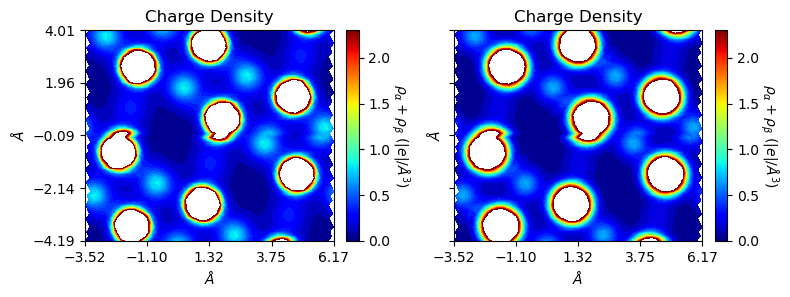
Plot 2D charge/spin densities
The plot_2D() method helps to visualize the charge / spin densities.
Plot them together with default setups (color-filled contour plot):
[7]:
from CRYSTALpytools.electronics import ChargeDensity

fig = ChargeDensity.from_file('dens_hematite.f25',
                              output='dens_hematite.out').plot_2D()
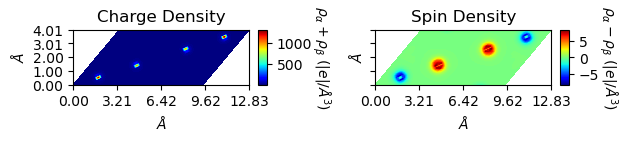
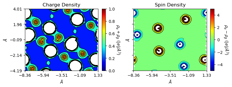
Not nice. Change the settings of levels for plot levels and range, and figsize for figure size.
[8]:
from CRYSTALpytools.electronics import ChargeDensity
import numpy as np

chglevel = np.log10(np.linspace(1, 10, 100))
spinlevel = np.linspace(-5, 5, 100)

chg = ChargeDensity.from_file('dens_hematite.f25', output='dens_hematite.out')
fig = chg.plot_2D(levels=[chglevel, spinlevel], figsize=[10, 5])
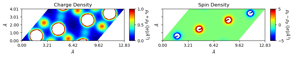
In this example, the plot is non-orthogonal. The user can get orthogonal plot by setting rectangle=True. The cmode moves the non-orthogonal part on the right to the left hand side, i.e., similar to the ‘RECTANGU’ keyword of ‘MAPNET’ (see CRYSTAL manual).
[9]:
from CRYSTALpytools.electronics import ChargeDensity
import numpy as np

chglevel = np.log10(np.linspace(1, 10, 100))
spinlevel = np.linspace(-5, 5, 100)

chg = ChargeDensity.from_file('dens_hematite.f25', output='dens_hematite.out')
fig = chg.plot_2D(levels=[chglevel, spinlevel], figsize=[8, 5], rectangle=True)
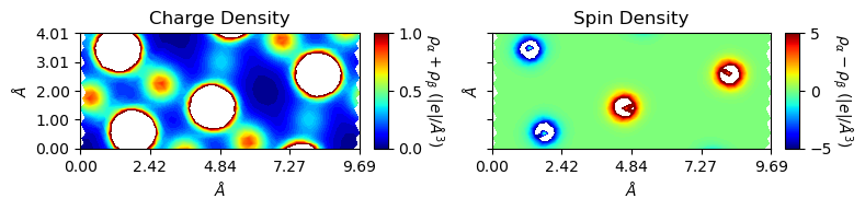
The monovacancy is off-center after rectangle plotting. The user can modify periodicity by setting a_range and b_range. Both of them uses fractional coordinates of plot base vector. If they are used with rectangle=True, that refers to the old, non-orthogonal base vectors. Coordinates of the original plotting window are kept.
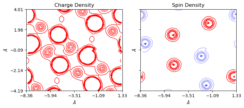
By setting lineplot=True and colorplot=False, contour lines is plotted. If both are ‘True’, contour lines are overlapped with color plots (not looking good with this example). Solid lines for positive values and 0 (doubled width). Dotted lines for negative values.
[10]:
from CRYSTALpytools.electronics import ChargeDensity
import numpy as np

chglevel = np.log10(np.linspace(1, 10, 10))
spinlevel = np.linspace(-5, 5, 10)

chg = ChargeDensity.from_file('dens_hematite.f25', output='dens_hematite.out')
fig = chg.plot_2D(levels=[chglevel, spinlevel], figsize=[8, 6], lineplot=True, colorplot=True,
                  a_range=[-0.5, 0.5], b_range=[-1, 1], rectangle=True)
It is also possible to get color-coded lines for contourplots with lineplot=True and colorplot=False. Positive values are denoted by solid red lines and negative by dotted blue lines. 0 is denoted by the solid black lines with doubled width.
[11]:
from CRYSTALpytools.electronics import ChargeDensity
import numpy as np

chglevel = np.log10(np.linspace(1, 10, 10))
spinlevel = np.linspace(-5, 5, 10)

chg = ChargeDensity.from_file('dens_hematite.f25', output='dens_hematite.out')
fig = chg.plot_2D(levels=[chglevel, spinlevel], figsize=[8, 6], lineplot=True, colorplot=False,
                  a_range=[-0.5, 0.5], b_range=[-1, 1], rectangle=True)
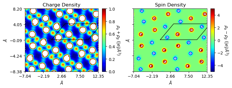
With a_range and b_range, one can also plot supercells. Set edgeplot=True to mark unit plot window boundaries at origin (0,0,0,), which is not influanced by ‘range’ or ‘rectangle’ options.
[12]:
from CRYSTALpytools.electronics import ChargeDensity
import numpy as np

chglevel = np.log10(np.linspace(1, 10, 100))
spinlevel = np.linspace(-5, 5, 100)

chg = ChargeDensity.from_file('dens_hematite.f25', output='dens_hematite.out')
fig = chg.plot_2D(levels=[chglevel, spinlevel], figsize=[8, 6],
                  a_range=[0, 2], b_range=[-2, 2],
                  rectangle=True, edgeplot=True)
Plot 3D charge/spin densities
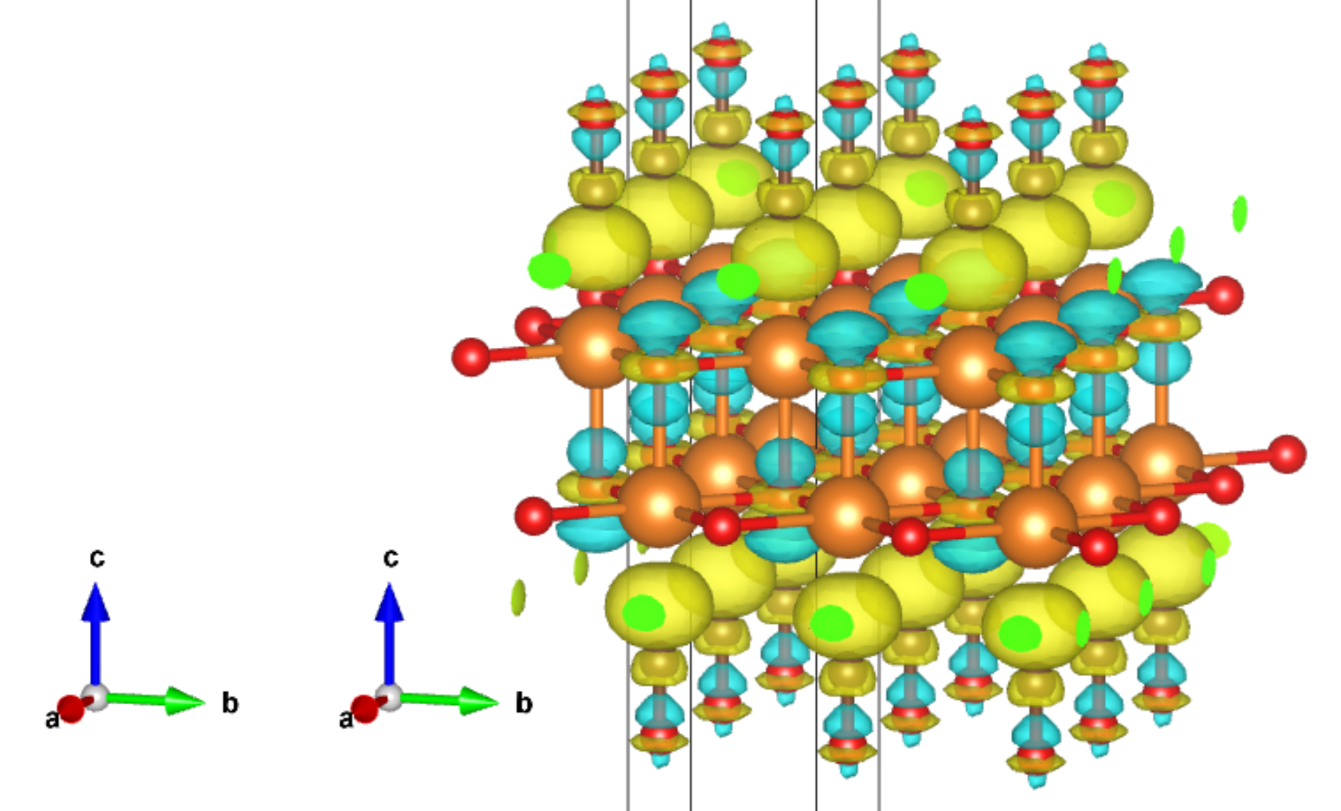
The plot_3D() method helps to visualize the 2D/3D charge / spin densities with 3D structures. It requires MayaVi, which is not in the dependency list of CRYSTALpytools.
Plot charge densities of hematite as 3D isosurfaces.
[13]:
from CRYSTALpytools.electronics import ChargeDensity

obj = ChargeDensity.from_file('dens_hematite_chg.cube',
                              output='dens_hematite.out')
obj.plot_3D(isovalue=[0.1, 0.2, 0.5, 1.0],
            opacity=0.2,
            scale=1.0) # 'scale' is for bond searching
/home/huanyu/apps/anaconda3/envs/crystal_py3.9/lib/python3.9/site-packages/CRYSTALpytools/electronics.py:1232: UserWarning: Inconsistent geometries are given in output and CUBE files, using the one from output.
  cls = Properties_output(output).read_ECH3(*files, method=method)
MayaVi output
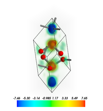
Plot spin densities of hematite as 3D volume data. Use the grid_display_range to change the display range of the data grid.
NOTE In some cases it might be very time consuming!
[14]:
from CRYSTALpytools.electronics import ChargeDensity

obj = ChargeDensity.from_file('dens_hematite_spin.cube',
                              output='dens_hematite.out')
obj.plot_3D(volume_3d=True, vmin=-1, vmax=1,
            grid_display_range=[[0, 1], [0, 1], [0,1]],
            scale=1.0) # 'scale' is for bond searching
/home/huanyu/apps/anaconda3/envs/crystal_py3.9/lib/python3.9/site-packages/CRYSTALpytools/electronics.py:1232: UserWarning: Inconsistent geometries are given in output and CUBE files, using the one from output.
  cls = Properties_output(output).read_ECH3(*files, method=method)
MayaVi output
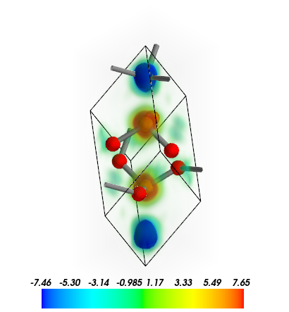
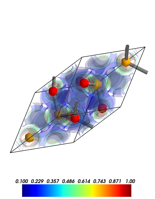
plot_3D can also be used to visualize 2D data planes, in which case the 3D structure is plotted.
Plot spin densities of hematite in 2D plane. Use the display_range to change the display range of the structure. Use contour_2d=True to plot contour lines.
[15]:
from CRYSTALpytools.electronics import ChargeDensity

obj = ChargeDensity.from_file('dens_hematite.f25',
                              output='dens_hematite.out')
obj.plot_3D(option='spin',
            isovalue=[-1, -0.5, -0.25, 0, 0.25, 0.5, 1],
            contour_2d=True,
            interp='linear',
            interp_size=2,
            display_range=[[0, 2], [0, 2], [0,2]],
            scale=1.0) # 'scale' is for bond searching
MayaVi output:
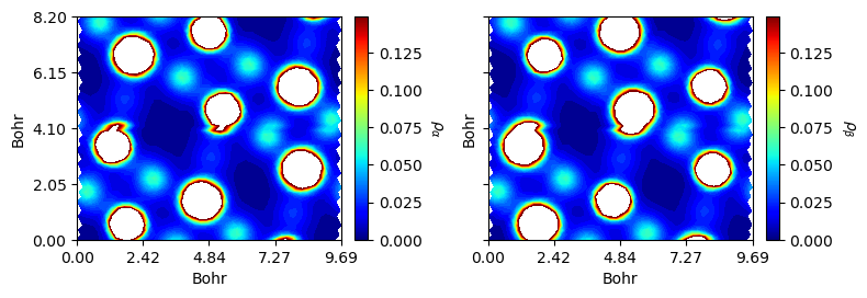
Analysis
As has illustrated above, the subtract() method helps to generate difference maps. The alpha_beta() method splits \(\alpha\) and \(\beta\) densities into the original charge and spin densities.
[16]:
from CRYSTALpytools.electronics import ChargeDensity
import numpy as np

chglevel = np.log10(np.linspace(1, 10, 100)) * 0.53**3 # roughly convert AA^-3 to Bohr^-3

chg = ChargeDensity.from_file('dens_hematite.f25', method='alpha_beta',
                              output='dens_hematite.out')
fig = chg.plot_2D(unit='a.u.', levels=[chglevel, chglevel], figsize=[8, 6],
                  cbar_label=[r'$\rho_{\alpha}$', r'$\rho_{\beta}$'],
                  b_range=[0, 2], rectangle=True, title=None)
Conversion to XSF
The to_xsf() method helps to write 2D/3D charge/spin densities into the XCrySDen XSF format for visualization and analysis. Such file format is accepted by many popular modelling software such as XCrySDen, VMD and VESTA.
NOTE
For 3D data grid, if CUBE file(s) are read without output, the XSF file output has the 3D ‘CRYSTAL’ periodicity. As far as the authors have been aware of, this only causes Segmentation Fault of XCrySDen 1.6.2 when dealing with low dimensional systems. Available solution includes:
including output file
using other software such as VESTA
changing the keyword manually.
Convert the same system into XSF format with 2D data grid.
[17]:
from CRYSTALpytools.electronics import ChargeDensity

chg = ChargeDensity.from_file('dens_hematite.f25', output='dens_hematite.out')
chg.to_xsf('dens_hematite.xsf')
Visualize charge densities in XCrySDen.
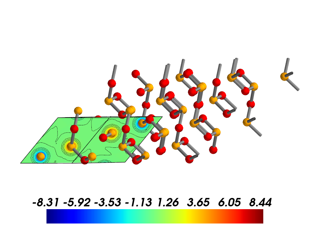
Get charge density difference before and after CO adsoprtion onto the MgO \((001)\) 2 layers slab.
[19]:
from CRYSTALpytools.electronics import ChargeDensity

dchg = ChargeDensity.from_file('dens_MgOCO.cube',
                               'dens_MgO.cube',
                               'dens_CO.cube',
                               output='dens_MgOCO.out',
                               method='subtract')
dchg.to_xsf('dens_dMgOCO.xsf')
Visualize charge density difference in VESTA. The cell has been expanded 3 times in both directions.
The ‘plot.plot_ECHG()’ function
The plot.plot_ECHG() function enables a higher-level of plotting. It accepts extendable length of ‘fort.25’ files or ChargeDensity objects.
Single-system charge / spin density.
By default the charge / spin densities of a single sysmtem is plotted, as the example showed above.
Multi-system charge / spin densities
plot_ECHG() can read entries of arbitrary length and return to the matplotlib Figure object with subplots. For comparison, the uniform scale can be used by setting levels.
[20]:
from CRYSTALpytools.plot import plot_ECHG
import numpy as np

chglevel = np.log(np.linspace(1, 10, 100))
files = ['dens_hematite.f25', 'dens_hematitePATO.f25']

figs = plot_ECHG(*files, option='charge', levels=chglevel,
                 rectangle=True, figsize=[8, 6], b_range=[-1, 1])
/home/huanyu/apps/anaconda3/envs/crystal_py3.9/lib/python3.9/site-packages/CRYSTALpytools/electronics.py:1230: UserWarning: Properties output file not found: Only the first 1 (2) density map(s) will be read for spin=1(2).
  cls = Properties_output(output).read_ECHG(*files, method=method)
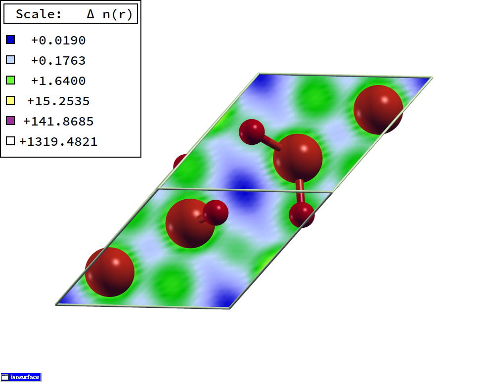
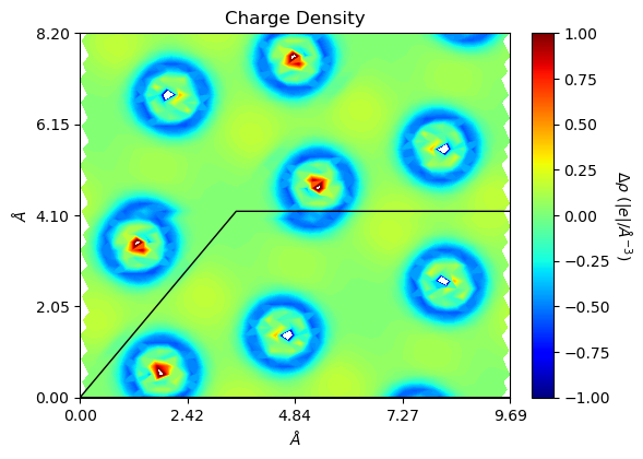
With option='diff', the user can quickly plot charge difference maps. It returns to non spin-polarized solution (obj.spin=1) as only charge density difference is considered.
[21]:
from CRYSTALpytools.plot import plot_ECHG
import numpy as np

chglevel = np.linspace(-1, 1, 100)
files = ['dens_hematite.f25', 'dens_hematitePATO.f25']

figs = plot_ECHG(*files, option='diff', levels=chglevel, rectangle=True,
                 b_range=[0, 2], edgeplot=True, figsize=[6, 6],
                 add_title=False, cbar_label=r'$\Delta\rho$ ($|e|/\AA^{-3}$)')
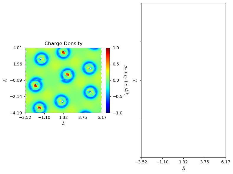
If the object contains both charge and ‘PATO’ charge, and was generated with ‘subtract’ method, plot it with ‘charge’. Otherwise a warning message is generated.
[22]:
from CRYSTALpytools.electronics import ChargeDensity
from CRYSTALpytools.plot import plot_ECHG
import numpy as np

chglevel = np.linspace(-1, 1, 100)
dchg = ChargeDensity.from_file('dens_hematite.f25', output='dens_hematite.out',
                               method='subtract')
fig = plot_ECHG(dchg, levels=chglevel, figsize=[8, 6], b_range=[-1, 1],
                rectangle=True)
/home/huanyu/apps/anaconda3/envs/crystal_py3.9/lib/python3.9/site-packages/CRYSTALpytools/plot.py:173: UserWarning: Spin options not available to non spin-polarized cases.
  fig = o.plot_2D(unit, 'both', levels, lineplot, linewidth, isovalues,
The following code block is only used to generate a nice thumbnail for the example gallary.
This is the end of the example notebook. For more details, please refer to the API documentations.
[1]:
import matplotlib.pyplot as plt
fig, ax = plt.subplots()
ax.imshow(plt.imread("./dens_hematite3Dvol.png"))
ax.axis('off')
[1]:
(-0.5, 409.5, 442.5, -0.5)